Plot of the orientation tensor for short fiber composites

This example shows how to reconstruct and plot the components of the fiber orientation tensor in the global coordinate system.

For more details about the fiber orientation tensor, refer to the Short Fiber Composites help.

Note

To run this example you first need to install the SciPy package.

Set up analysis

Setting up the analysis consists of loading Ansys libraries, connecting to the DPF server, and retrieving the example files.

Load Ansys libraries.

import ansys.dpf.core as dpf
import numpy as np
from scipy.spatial.transform import Rotation

from ansys.dpf.composites.example_helper import get_short_fiber_example_files
from ansys.dpf.composites.server_helpers import connect_to_or_start_server

Start a DPF server and copy the example files into the current working directory. These files are needed:

• Mechanical APDL result (RST) file containing the simulation results

• Mechanical APDL input file (DS.DAT) containing the fiber orientation tensor data

server = connect_to_or_start_server()
composite_files_on_server = get_short_fiber_example_files(server, "short_fiber")

Set up data sources

Set up the data sources.

data_sources = dpf.DataSources()
data_sources.add_file_path(composite_files_on_server.dsdat, "dat")
data_sources.set_result_file_path(composite_files_on_server.rst)

Initialize DPF model

Initialize the DPF model.

model = dpf.Model(data_sources=data_sources)
mesh = model.metadata.meshed_region

Should your mesh contain both solid and shell elements, for visualization purposes it can be useful to scope the mesh to the solid ones.

# solid_scoping_op = dpf.operators.scoping.on_mesh_property(
#   property_name='solid_elements',
#   mesh=mesh,
# )
# solid_mesh = dpf.operators.mesh.from_scoping(
#   scoping=solid_scoping_op.outputs.mesh_scoping(),
#   mesh=model.metadata.mesh_provider,
# ).outputs.mesh()

Plot input data

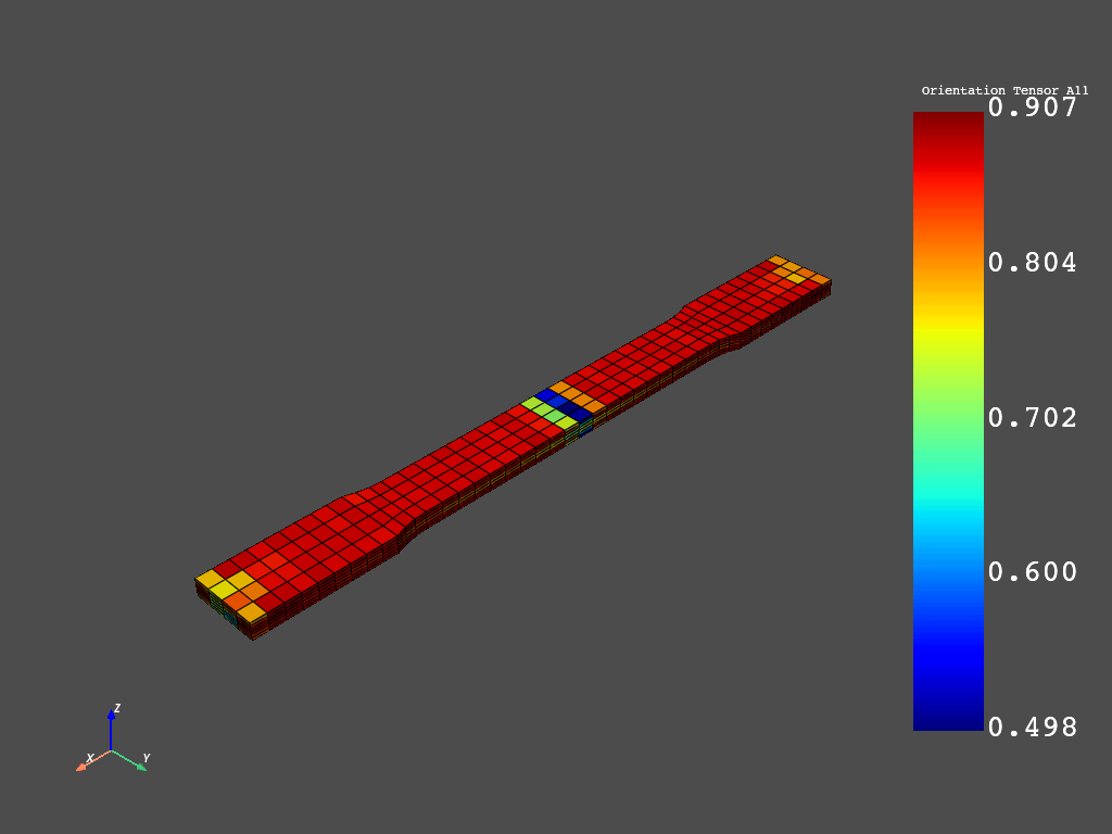
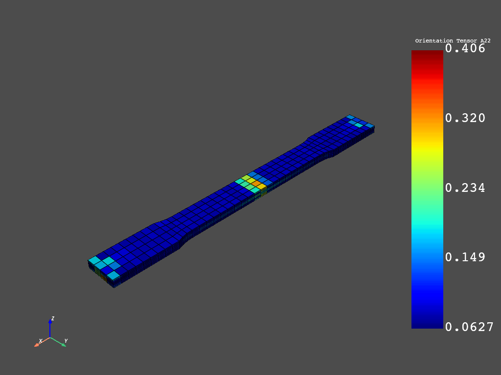
Plot the two largest eigenvalues (a11 and a22) of the fiber orientation tensor. Note that the plots reveal the presence of a weld line in the middle of the specimen.

field_variable_provider = dpf.Operator("composite::inistate_field_variables_provider")
field_variable_provider.inputs.data_sources(data_sources)
field_variable_provider.inputs.mesh(mesh)

field_variable_dict = {
    fv.name: fv for fv in field_variable_provider.outputs.fields_container.get_data()
}

A11_NAME = "Orientation Tensor A11"
A22_NAME = "Orientation Tensor A22"

a11 = field_variable_dict[A11_NAME]
a11.plot()

a22 = field_variable_dict[A22_NAME]
a22.plot()

• 
• 

Compute results

Reconstruct the fiber orientation tensor in the global coordinate system.

element_ids = a11.scoping.ids
# Alternatively, you could for instance scope to a named selection with
# >>> element_ids = model.metadata.meshed_region.named_selection('CENTER').ids

# Define the fiber orientation tensor in the global coordinate system
# as a symmetrical 3x3 tensor with components XX,YY,ZZ,XY,YZ,XZ.
fiber_orientation_tensor = dpf.fields_factory.create_tensor_field(
    num_entities=len(element_ids), location=dpf.locations.elemental
)

ele_orientation_op = dpf.operators.result.element_orientations(
    data_sources=data_sources, requested_location="Elemental", bool_rotate_to_global=False
)

euler_angles_field = ele_orientation_op.outputs.fields_container()[0]
for eid in element_ids:
    V = Rotation.from_euler(
        seq="ZXY", angles=euler_angles_field.get_entity_data_by_id(eid)[0], degrees=True
    ).as_matrix()
    d1 = a11.get_entity_data_by_id(eid)[0]
    d2 = a22.get_entity_data_by_id(eid)[0]
    D = np.diag([d1, d2, max(1.0 - d1 - d2, 0.0)])
    aRot = np.matmul(np.matmul(V, D), V.transpose())
    fiber_orientation_tensor.append(
        [aRot[0, 0], aRot[1, 1], aRot[2, 2], aRot[0, 1], aRot[1, 2], aRot[0, 2]], eid
    )

fiber_orientation_tensor_fc = dpf.operators.utility.field_to_fc(
    field=fiber_orientation_tensor
).outputs.fields_container()

Plot results

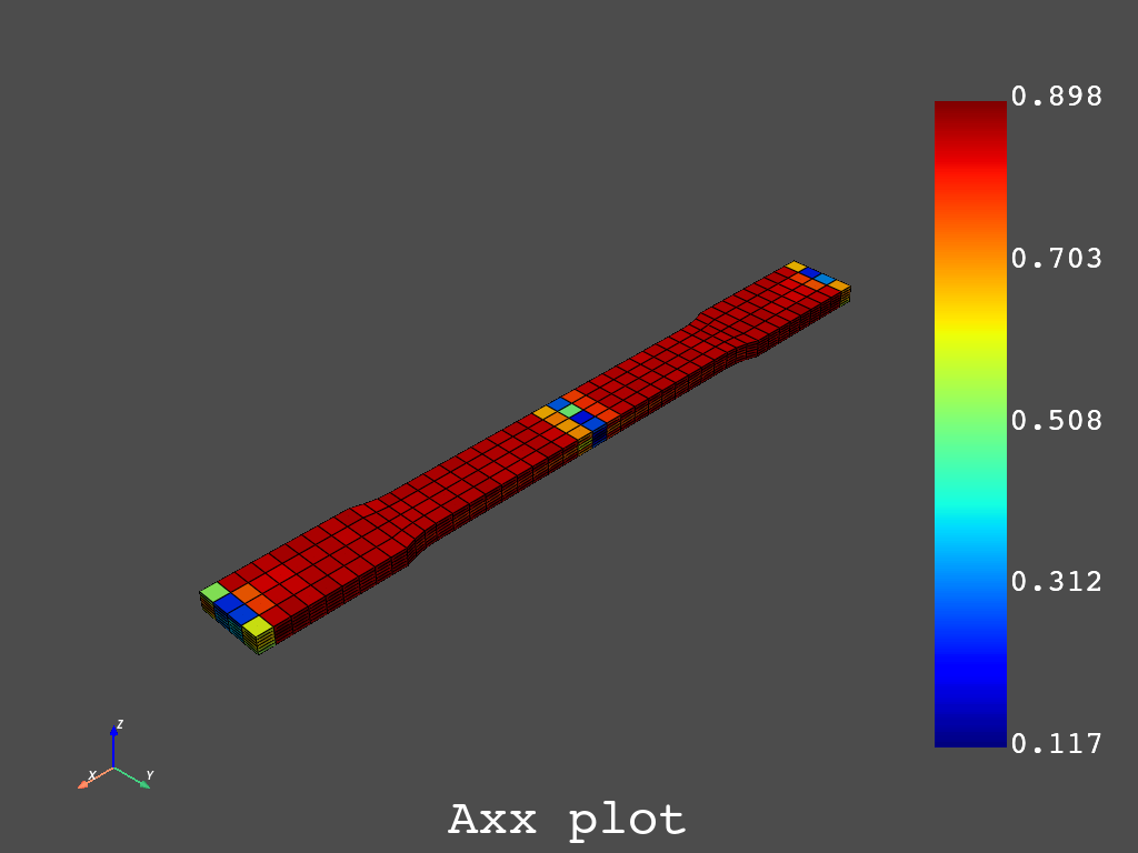
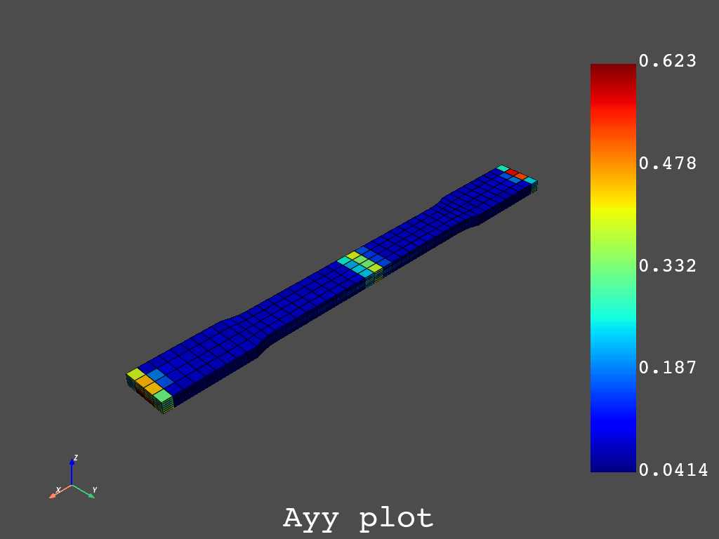
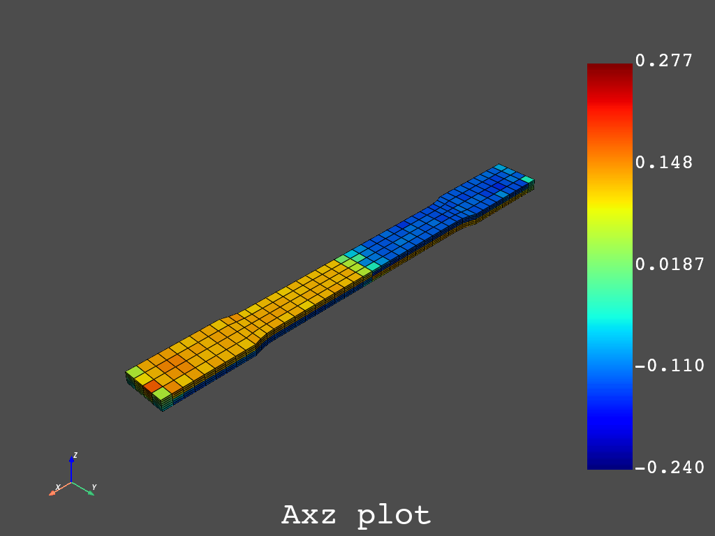
Plot some components of the fiber orientation tensor.

aXX = fiber_orientation_tensor_fc.select_component(0)[0]
aYY = fiber_orientation_tensor_fc.select_component(1)[0]
aXZ = fiber_orientation_tensor_fc.select_component(5)[0]

mesh.plot(aXX, title="Axx", text="Axx plot")
mesh.plot(aYY, title="Ayy", text="Ayy plot")
mesh.plot(aXZ, title="Axz", text="Axz plot")

• 
• 
•