Thermal analysis

This example shows how to evaluate a thermal analysis. The simulation’s thermal analysis results are also the input of a structural analysis. Therefore, the RST file contains temperature and structural results.

The example imitates a printed circuit board (PCB) that was modeled with Ansys Composites PrepPost (ACP), using the solid model feature to generate the volume mesh.

Descriptions of how to extract temperatures for a specific ply and material are provided.

Note

When using a Workbench project, use the get_composite_files_from_workbench_result_folder() method to obtain the input files.

Set up analysis

Setting up the analysis consists of loading the required modules, connecting to the DPF server, and retrieving the example files.

import ansys.dpf.core as dpf
import numpy as np

from ansys.dpf.composites.composite_model import CompositeModel
from ansys.dpf.composites.example_helper import get_continuous_fiber_example_files
from ansys.dpf.composites.layup_info import get_all_analysis_ply_names
from ansys.dpf.composites.ply_wise_data import SpotReductionStrategy, get_ply_wise_data
from ansys.dpf.composites.select_indices import get_selected_indices_by_dpf_material_ids
from ansys.dpf.composites.server_helpers import connect_to_or_start_server

server = connect_to_or_start_server()
composite_files = get_continuous_fiber_example_files(server, "thermal_solid")

Initialize the model

Initialize the composite model with the composite files and server. The model provides access to the mesh, results, lay-up, and materials.

composite_model = CompositeModel(composite_files, server)

Get temperature results

The temperatures are stored under structural_temperature.

temp_op = composite_model.core_model.results.structural_temperature()
temperatures_fc = temp_op.outputs.fields_container()

Get ply results

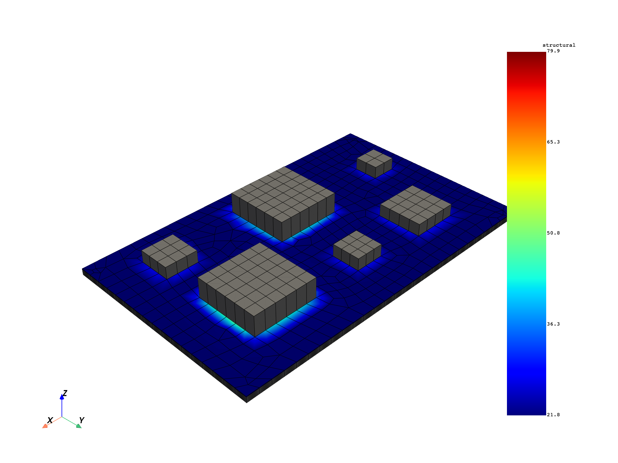
Extract the ply-wise results by passing the ply name to the function get_ply_wise_data().

all_ply_names = get_all_analysis_ply_names(composite_model.get_mesh())
print(all_ply_names)

# The component of the temperature is 0 which is the default value.
nodal_values = get_ply_wise_data(
    field=temperatures_fc,
    ply_name="P1L1__ModelingPly.8",
    mesh=composite_model.get_mesh(),
    spot_reduction_strategy=SpotReductionStrategy.MAX,
    requested_location=dpf.locations.nodal,
)

composite_model.get_mesh().plot(nodal_values)

Static Scene

Interactive Scene

['P1L1__p1_2_4_6', 'P1L1__p3', 'P1L1__ModelingPly.1', 'P1L1__p5', 'P1L1__ModelingPly.6', 'P1L1__ModelingPly.5', 'P1L1__ModelingPly.4', 'P1L1__ModelingPly.2', 'P1L1__ModelingPly.7', 'P1L1__ModelingPly.8', 'P1L1__ModelingPly.3']

Get results by material

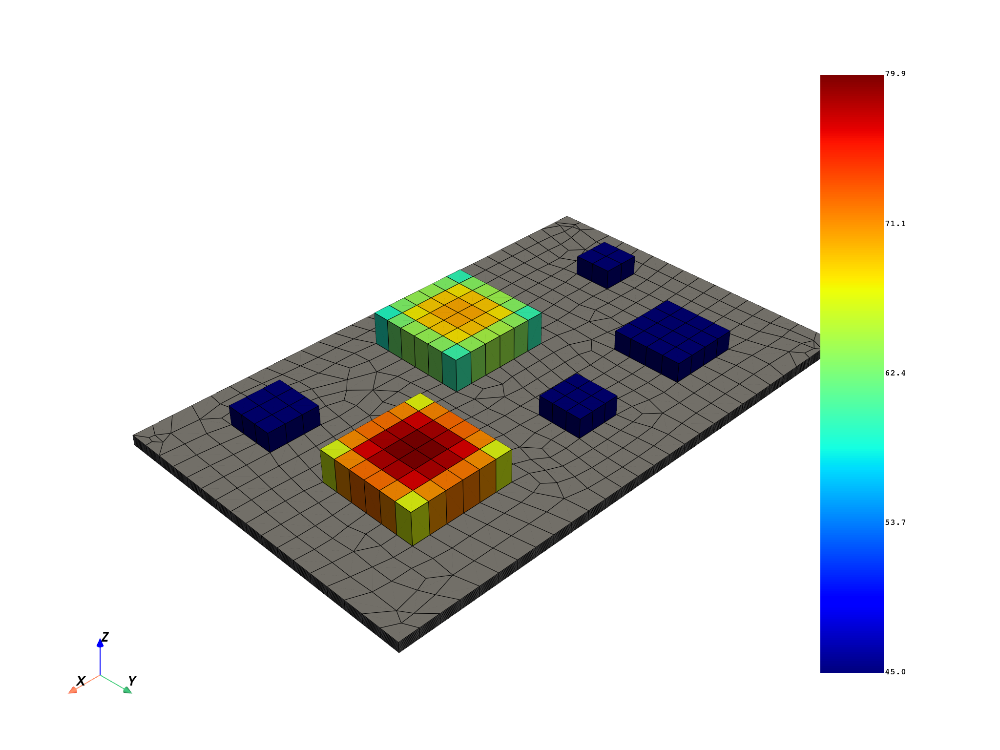
You can filter the results by material. In this example, the element-wise maximum temperature is extracted for the material Honeycomb Aluminum Alloy.

print(composite_model.material_names)
material_id = composite_model.material_names["Honeycomb Aluminum Alloy"]

# get the last result field
temperatures_field = temperatures_fc[-1]

material_result_field = dpf.field.Field(location=dpf.locations.elemental, nature=dpf.natures.scalar)
# performance optimization: use a local field instead of a field which is pushed to the server
with material_result_field.as_local_field() as local_result_field:
    element_ids = temperatures_field.scoping.ids

    for element_id in element_ids:
        element_info = composite_model.get_element_info(element_id)
        assert element_info is not None
        if material_id in element_info.dpf_material_ids:
            temp_data = temperatures_field.get_entity_data_by_id(element_id)
            selected_indices = get_selected_indices_by_dpf_material_ids(element_info, [material_id])

            value = np.max(temp_data[selected_indices])
            local_result_field.append([value], element_id)

composite_model.get_mesh().plot(material_result_field)

Static Scene

Interactive Scene

{'Honeycomb Aluminum Alloy': np.int32(1), 'UD Resin Epoxy/E-Glass': np.int32(2)}