Note
Go to the end to download the full example code.
LS-Dyna Bird Strike#
This example shows how to set up the composite model for a LSDyna analysis, how to post-process it and how to filter the results. The simulation uses SPH (Smooth Particle Hydrodynamics) to mimic a bird strike on a leading edge of a composite wing.
Additional steps are required to process LS-Dyna results if compared with a Mechanical APDL analysis.
- On the pre-processing side, these are:
The input file must be generated with WB LS Dyna
In WB Mechanical, enable the beta options and
Output Integration
Points Results for All ACP Plies
or manually set MAXINT of the keywordDATABASE_EXTENT_BINARYto the maximum number of plies.
- And these items must be considered on setting up the post-processing:
On initializing the composite model, these properties of
ContinuousFiberCompositesFilesmust be set:solver_typetoLSDYNAandsolver_input_filemust point to the keyword file (for instanceinput.k).The number of maximum integration points (MAXINT) has to be extracted from the keyword file. See
composite::ls_dyna_keyword_parseroperator.The results (stress, strain, history variable etc.) must be pre-processed to support ply-wise filtering and to make them consistent with the layup model. See
composite::ls_dyna_preparing_resultsoperator.
- Note:
Use the
get_composite_files_from_workbench_result_folder()to get the composite files from a WB LS-Dyna result folder. Setsolver_typetoLSDYNA.Only the first d3plot file must be passed to the composite model. The LSDyna reader will automatically pick up the other files.
Set up analysis#
Setup of the analysis and initialize the composite model.
import json

import ansys.dpf.core as dpf
from ansys.dpf.core import Operator, unit_systems

from ansys.dpf.composites.composite_model import CompositeModel
from ansys.dpf.composites.constants import Sym3x3TensorComponent
from ansys.dpf.composites.example_helper import get_continuous_fiber_example_files
from ansys.dpf.composites.ply_wise_data import SpotReductionStrategy, get_ply_wise_data
from ansys.dpf.composites.server_helpers import connect_to_or_start_server
server = connect_to_or_start_server()
composite_files_on_server = get_continuous_fiber_example_files(server, "lsdyna_bird_strike")

composite_model = CompositeModel(
    composite_files=composite_files_on_server,
    server=server,
    default_unit_system=unit_systems.solver_nmm,
)
Get all the time ids to read all time steps and to select the correct results.
time_freq_support = composite_model.core_model.metadata.time_freq_support
time_ids = [int(v) for v in time_freq_support.time_frequencies.scoping.ids]
Get displacements at the final time step
disp_result = composite_model.core_model.results.displacement()
displacement = disp_result.eval().get_field({"time": time_ids[-1]})
Read stresses in the material coordinate system
stress_operator = composite_model.core_model.results.stress()
stress_operator.inputs.bool_rotate_to_global(False)
Prepare data#
The LS Dyna results have to be pre-processed to support ply-wise
filtering because the data must be consistent with the layup
model. This pre-processing is based on the maximum
integration points (MAXINT) from the DATABASE_EXTENT_BINARY keyword.
This parameter can be extracted from the input file (input.k) with
the help of the composite::ls_dyna_keyword_parser operator.
def prepare_lsdyna_results(
    my_results_container: dpf.fields_container.FieldsContainer,
) -> dpf.fields_container.FieldsContainer:
    keyword_parser = Operator("composite::ls_dyna_keyword_parser")
    keyword_parser.inputs.data_sources(composite_model.data_sources.solver_input_file)
    keyword_parser.inputs.keyword("DATABASE_EXTENT_BINARY")
    keyword_options_as_json = json.loads(keyword_parser.outputs.keyword_options.get_data())

    # remove unneeded integration points for each element
    strip_operator = Operator("composite::ls_dyna_preparing_results")
    strip_operator.inputs.maxint(int(keyword_options_as_json["maxint"]))
    strip_operator.inputs.fields_container(my_results_container)
    strip_operator.inputs.mesh(composite_model.get_mesh())
    stripped_results_container = strip_operator.outputs.fields_container.get_data()

    return stripped_results_container


stripped_stress_container = prepare_lsdyna_results(
    stress_operator.outputs.fields_container.get_data()
)
Filter data by analysis ply#
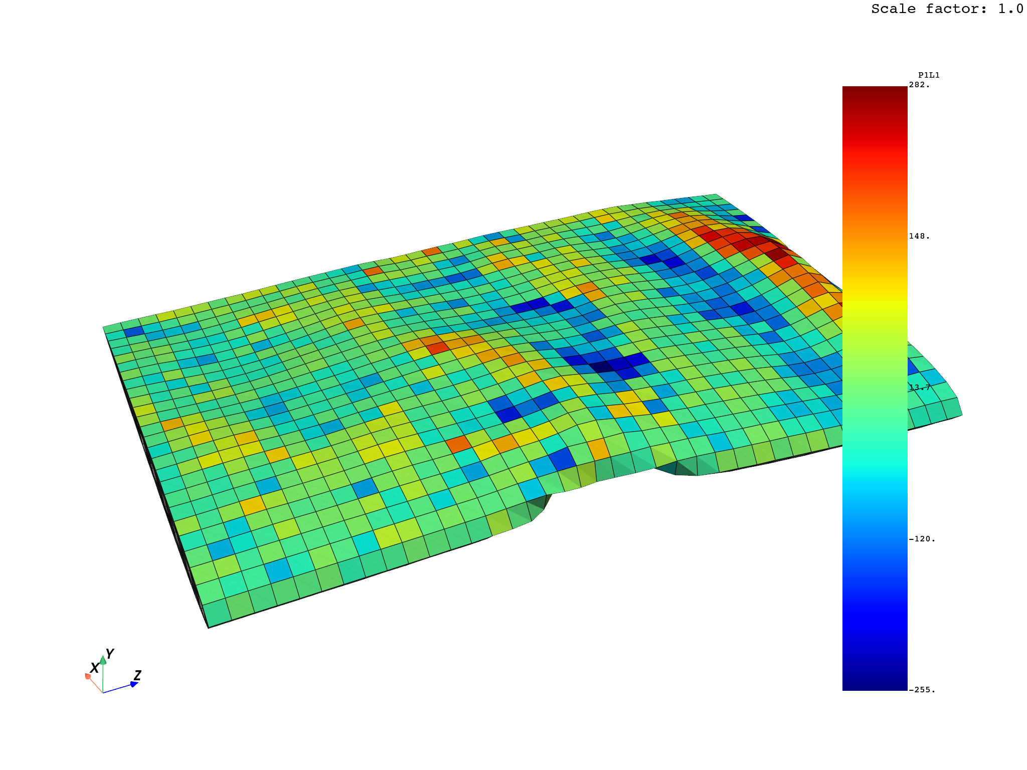
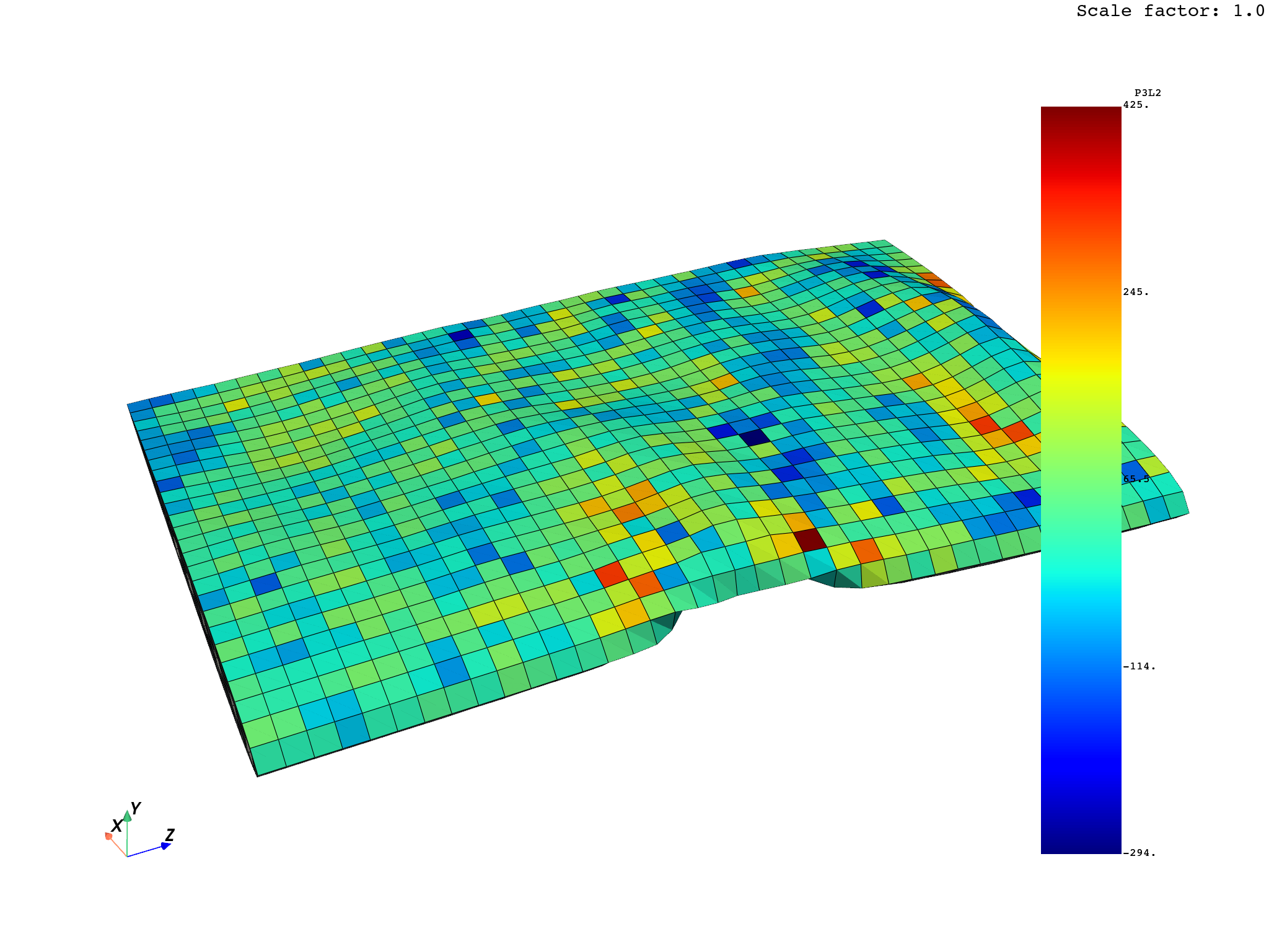
Print stresses of a few plies at the last time step. You can
use get_all_analysis_ply_names to list all available plies.
Note that one integration point per layer and element is available if
MAXINT is equal or greater than the number of layers.
stripped_stress_field = stripped_stress_container.get_field({"time": time_ids[-1]})
camera = [
    (-1589.7832333411716, 1670.8197500164952, -328.2144469600579),
    (493.2896802711351, 0.2085447040423768, 763.1274012915459),
    (0.5149806660541146, 0.8152207788520537, 0.26497168776741287),
]

for ply_name in ["P1L1__ModelingPly.1", "P3L2__ModelingPly.1"]:
    print(f"Plotting s1 of ply {ply_name}")
    elemental_values = get_ply_wise_data(
        field=stripped_stress_field,
        ply_name=ply_name,
        mesh=composite_model.get_mesh(),
        component=Sym3x3TensorComponent.TENSOR11,
        spot_reduction_strategy=SpotReductionStrategy.MAX,
        requested_location=dpf.locations.elemental,
    )

    composite_model.get_mesh().plot(
        field_or_fields_container=elemental_values,
        deform_by=displacement,
        cpos=camera,
    )


Plotting s1 of ply P1L1__ModelingPly.1
Plotting s1 of ply P3L2__ModelingPly.1
Plot history variables#
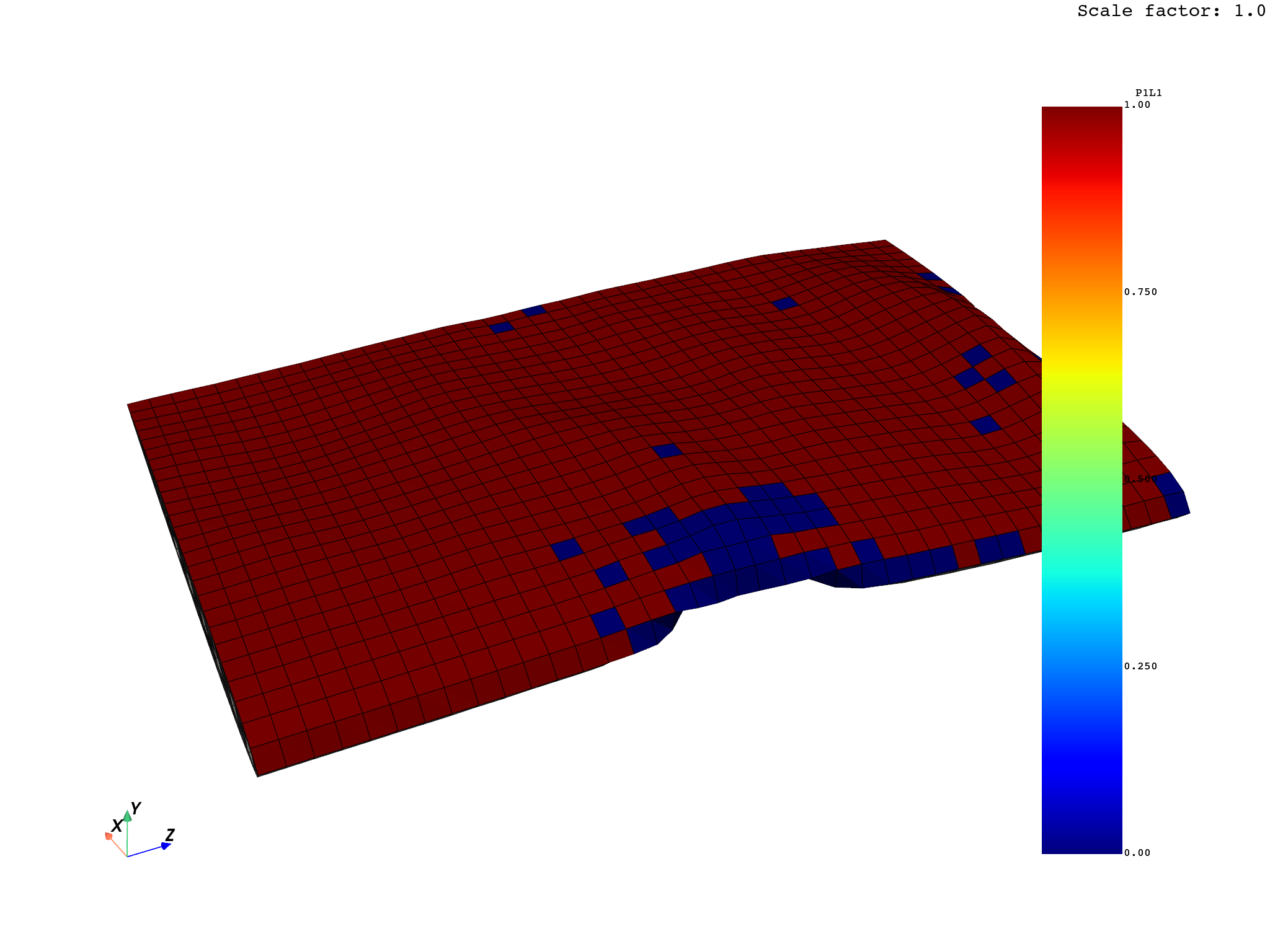
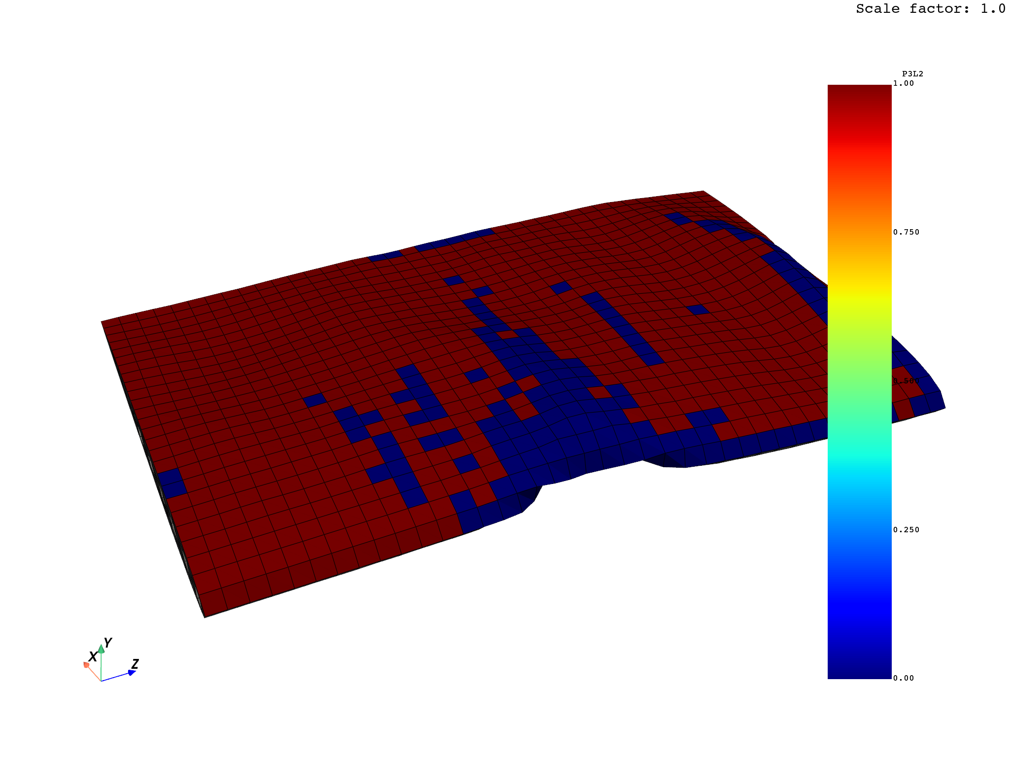
The same procedure can be applied to history variables. In this example, the 2nd history variable (compressive fiber mode) is plotted. 1 stands for elastic, 0 means failed.
hv_operator = dpf.Operator("lsdyna::d3plot::history_var")
hv_operator.inputs.data_sources(composite_model.data_sources.result_files)
hv_operator.inputs.time_scoping(time_ids)

stripped_hv_container = prepare_lsdyna_results(hv_operator.outputs.history_var.get_data())
stripped_hv_field = stripped_hv_container.get_field({"time": time_ids[-1], "ihv": 2})

for ply_name in ["P1L1__ModelingPly.1", "P3L2__ModelingPly.1"]:
    print(f"Plotting history variable 2 of ply {ply_name}")
    elemental_values = get_ply_wise_data(
        field=stripped_hv_field,
        ply_name=ply_name,
        mesh=composite_model.get_mesh(),
        component=0,
        spot_reduction_strategy=SpotReductionStrategy.MAX,
        requested_location=dpf.locations.elemental,
    )

    composite_model.get_mesh().plot(
        field_or_fields_container=elemental_values,
        deform_by=displacement,
        cpos=camera,
    )


Plotting history variable 2 of ply P1L1__ModelingPly.1
Plotting history variable 2 of ply P3L2__ModelingPly.1
Total running time of the script: (0 minutes 13.927 seconds)

