Evaluate fatigue for a composite plate

This example shows how to evaluate fatigue for a flat plate. It shows how you can use PyPDF Composites to select specific layers and define a custom combination method. For this example, the custom combination method is stress in fibre direction.

A random load time series is created. Taking into account that the load is assumed proportional, rainflow counting is applied to the load time series. Load ranges are then applied on the stress combination method, and damage is evaluated by using a dummy S-N curve.

Be aware that the fatpack package is not developed by Ansys, so it is the responsibility of the user to verify that it works as expected. For more information, see the fatpack package,

Set up analysis

Setting up the analysis consists of loading the required modules, connecting to the DPF server, and retrieving the example files.

Load Ansys libraries and numpy, matplotlib and fatpack

import ansys.dpf.core as dpf
import fatpack
import matplotlib.pyplot as plt
import numpy as np

from ansys.dpf.composites.composite_model import CompositeModel
from ansys.dpf.composites.constants import Sym3x3TensorComponent
from ansys.dpf.composites.example_helper import get_continuous_fiber_example_files
from ansys.dpf.composites.layup_info import AnalysisPlyInfoProvider
from ansys.dpf.composites.select_indices import get_selected_indices_by_analysis_ply
from ansys.dpf.composites.server_helpers import connect_to_or_start_server

Start a DPF server and copy the example files into the current working directory.

server = connect_to_or_start_server()
composite_files_on_server = get_continuous_fiber_example_files(server, "fatigue")

Create a composite model

composite_model = CompositeModel(composite_files_on_server, server)

Read stresses and define a specific layer and a component of stress tensor

Read stresses

stress_operator = composite_model.core_model.results.stress()
stress_operator.inputs.bool_rotate_to_global(False)
stress_fc = stress_operator.get_output(pin=0, output_type=dpf.types.fields_container)
stress_field = stress_fc.get_field_by_time_id(1)

Select layer P1L1__ModelingPly.2

analysis_ply_info_provider = AnalysisPlyInfoProvider(
    mesh=composite_model.get_mesh(), name="P1L1__ModelingPly.2"
)

Select Sigma11 as the combination method

component = Sym3x3TensorComponent.TENSOR11

Load time series and apply rainflow counting

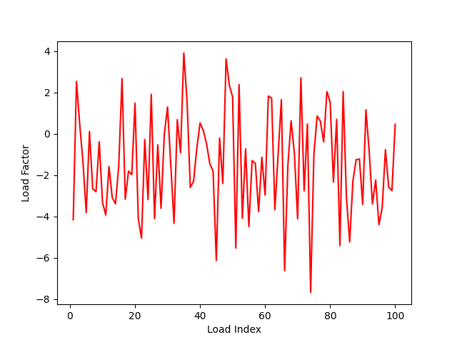
A random time series is created. Load is assumed proportional, so rainflow counting can be directly done on the load time series to get the load ranges. No mean stress correction is applied.

number_of_times = 100
load_factor_time_series = np.random.normal(-1, 2.5, size=number_of_times)
x = np.linspace(1, number_of_times, number_of_times)
plt.xlabel("Load Index")
plt.ylabel("Load Factor")
plt.plot(x, load_factor_time_series, color="red")

[<matplotlib.lines.Line2D object at 0x7f753b510640>]

Fatpack package is used for doing the rainflow counting

load_range_factors = fatpack.find_rainflow_ranges(load_factor_time_series)

S-N curve

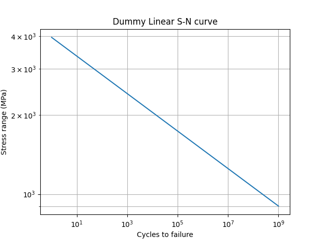
A dummy S-N curve is created. Note that this curve is not based on any experimental data. Sc is chosen to be twice the orthotropic stress limit in the fiber direction. and Nc is set to 1.

Sc = 2 * 1979
Nc = 1
s_n_curve = fatpack.LinearEnduranceCurve(Sc)
# Value for UD materials
s_n_curve.m = 14
s_n_curve.Nc = Nc

N = np.logspace(0, 9, 1000)
S = s_n_curve.get_stress(N)
line = plt.loglog(N, S)
plt.grid(which="both")
plt.title("Dummy Linear S-N curve")
plt.xlabel("Cycles to failure")
plt.ylabel("Stress range (MPa)")

Text(15.914246690538194, 0.5, 'Stress range (MPa)')

Damage evaluation

Stress S11 at time 1 and layer P1L1__ModelingPly.2 are read for each load range. Its damage is evaluated using the dummy S-N curve.

damage_result_field = dpf.field.Field(location=dpf.locations.elemental, nature=dpf.natures.scalar)

with damage_result_field.as_local_field() as local_result_field:
    element_ids = analysis_ply_info_provider.property_field.scoping.ids

    for element_id in element_ids:
        stress_data = stress_field.get_entity_data_by_id(element_id)
        element_info = composite_model.get_element_info(element_id)
        assert element_info is not None
        selected_indices = get_selected_indices_by_analysis_ply(
            analysis_ply_info_provider, element_info
        )
        # Load Range scaled by S11
        s_11 = max(stress_data[selected_indices][:, component])
        stress_ranges = load_range_factors * s_11
        fatigue_damage = s_n_curve.find_miner_sum(stress_ranges)
        local_result_field.append([fatigue_damage], element_id)

Plot damage

composite_model.get_mesh().plot(damage_result_field, text="Fatigue Damage")

Static Scene

Interactive Scene

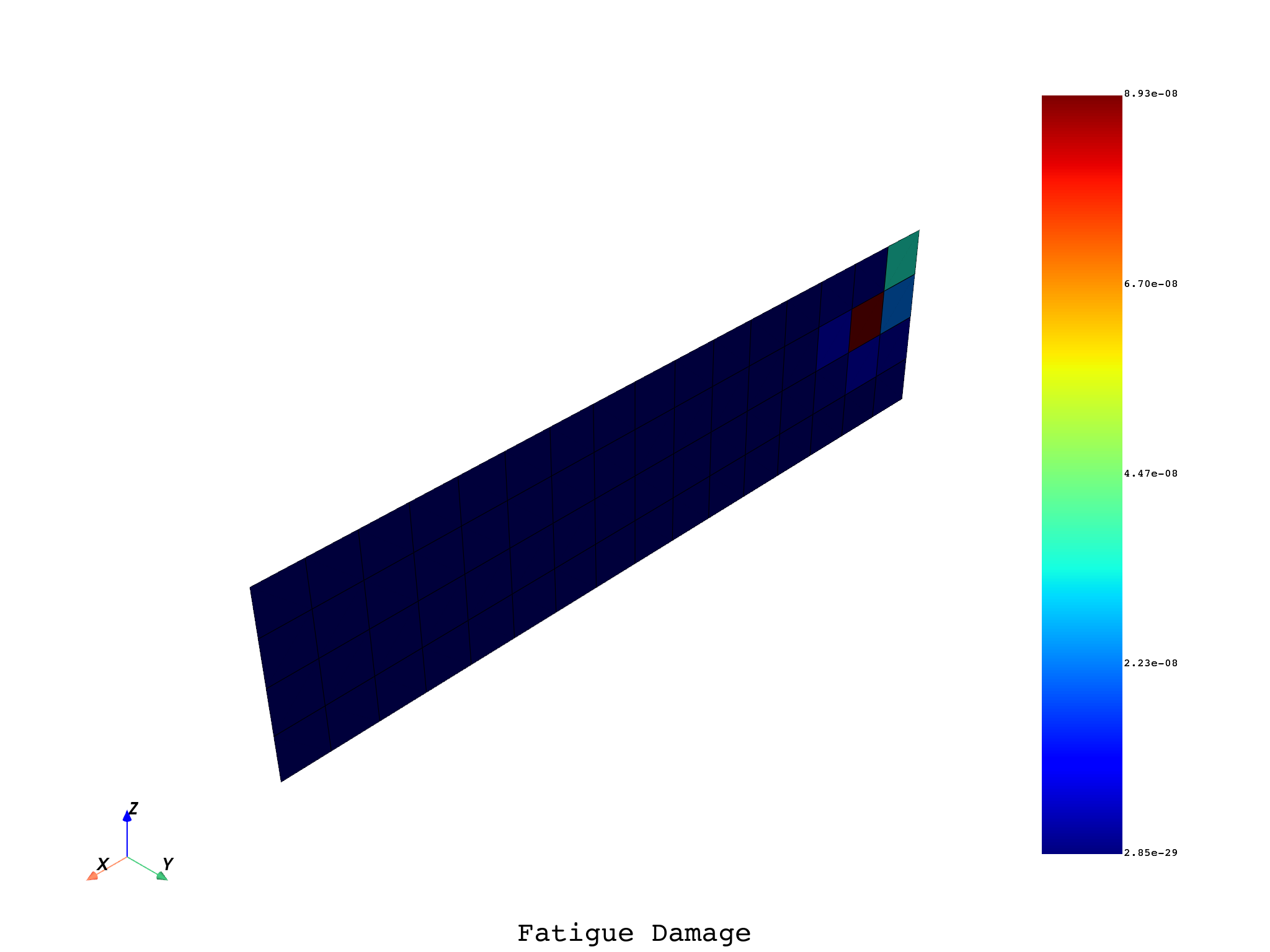
Identify the element with the maximum damage

maximum_element_scoping = damage_result_field.max().scoping
max_element_id = maximum_element_scoping[0]
print(f"The element with highest damage is {max_element_id}.")
print(f"The highest damage value is {damage_result_field.max().data[0]}.")

The element with highest damage is 27.
The highest damage value is 8.930735411967954e-08.